Maybe some friends still don’t know how to insert radar chart in office2007 Excel? Then the editor will bring you office2007 Tutorial on inserting a radar chart into Excel. Friends in need should come and take a look.
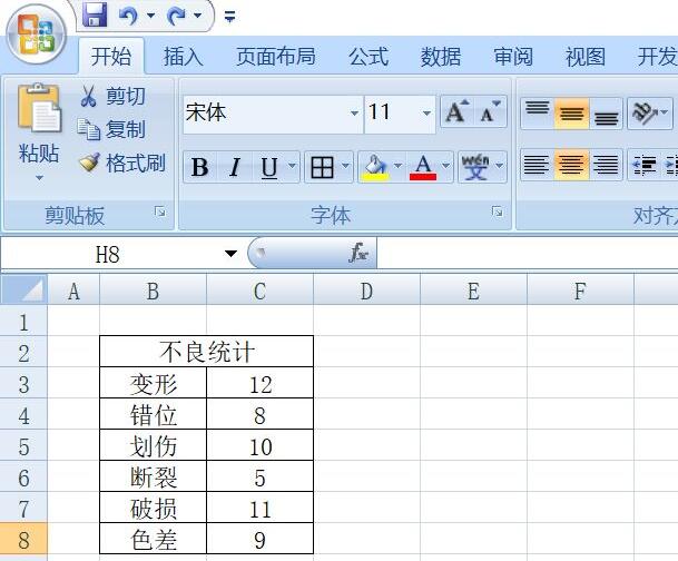
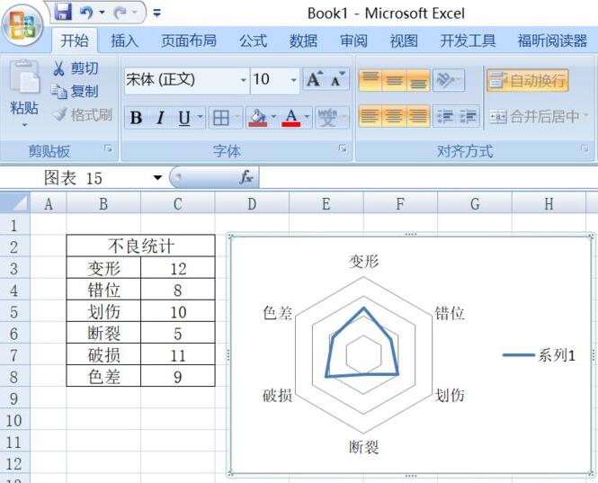
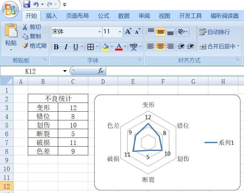
First, open an office 2007 Excel document, as shown in the figure, enter the relevant numbers and create a table;
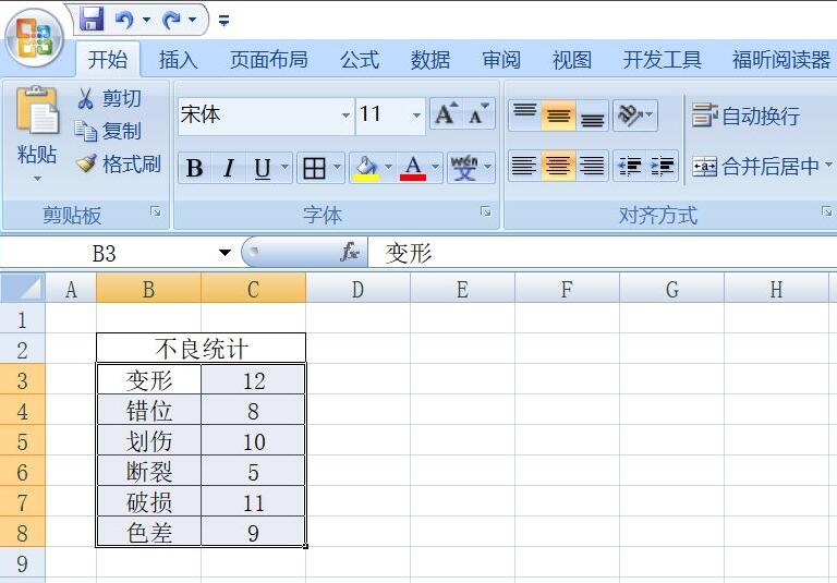
Then, select the cell of the bad item, as shown in the figure;
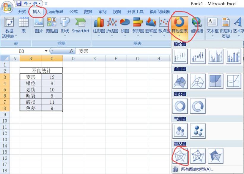
Then, click Insert, other icons, and the first icon of the radar chart, as shown in the figure;
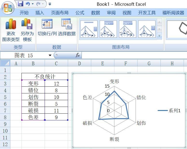
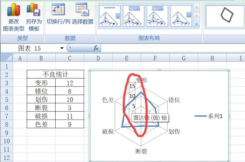
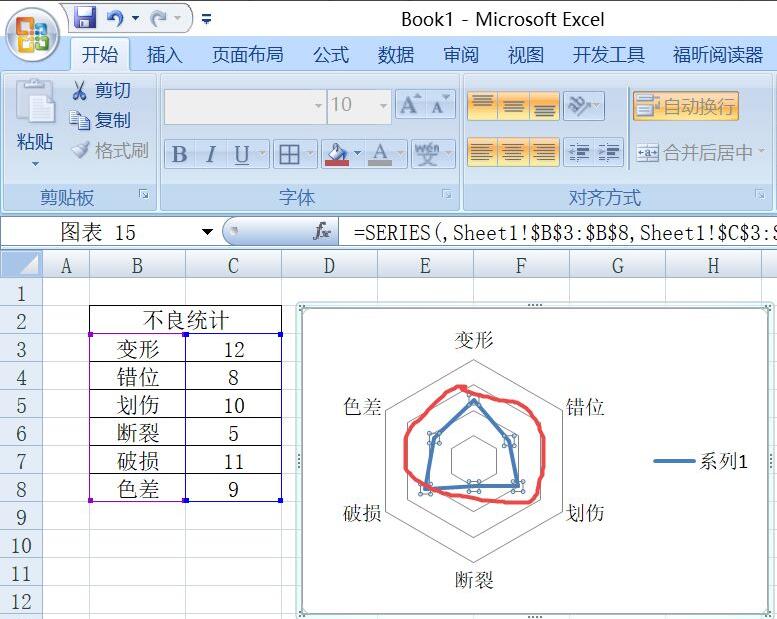
Then, the interface pops up as shown in the picture. Shrink the chart a little and place it in the lower right corner of the chart. When the shape is shown diagonally up and down, hold down the left button and drag it diagonally upward to zoom out. After zooming out, we move to the vicinity of the data value, as shown in the picture;
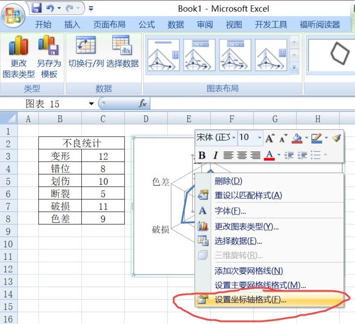
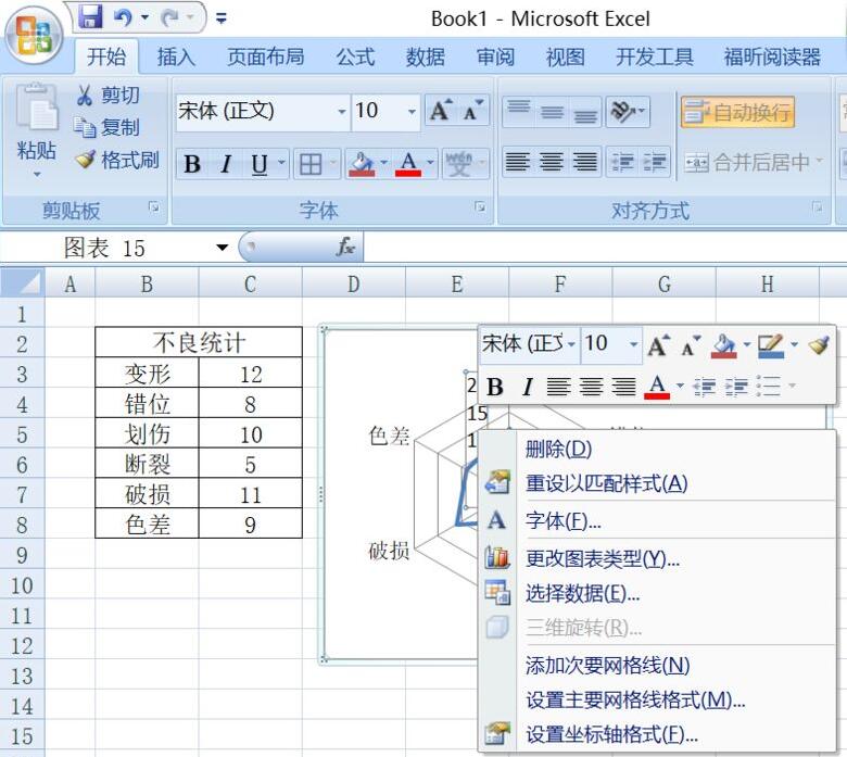
Left-click on the axis value, then select right-click, the interface will pop up, and select Set Axis Format;
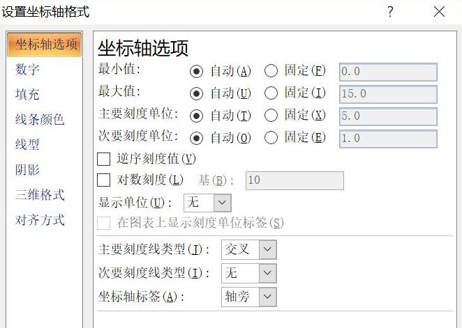
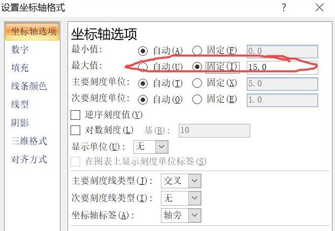
The pop-up interface is as shown in the figure. We will automatically change the maximum value to fixed, as shown in the figure;
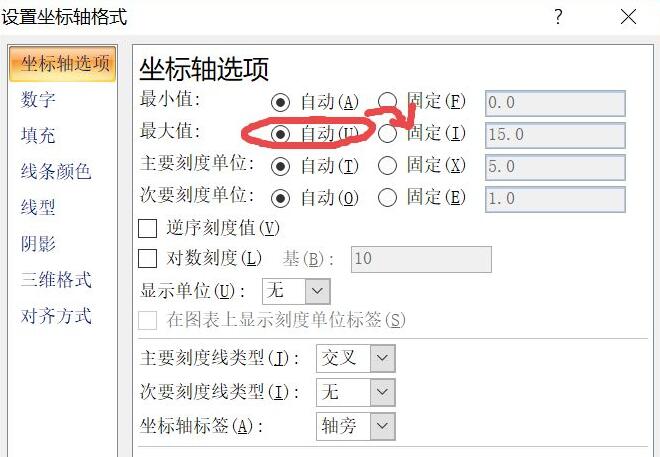
Change the value 15 inside to 20, and press End to close;
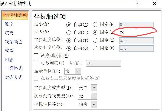
Right-click and select Delete; because our maximum value is 12, and the system’s automatic value is 15, when we add data labels later, the font and data labels will be superimposed, affecting viewing, so here we change the maximum value of the axis to a larger value.
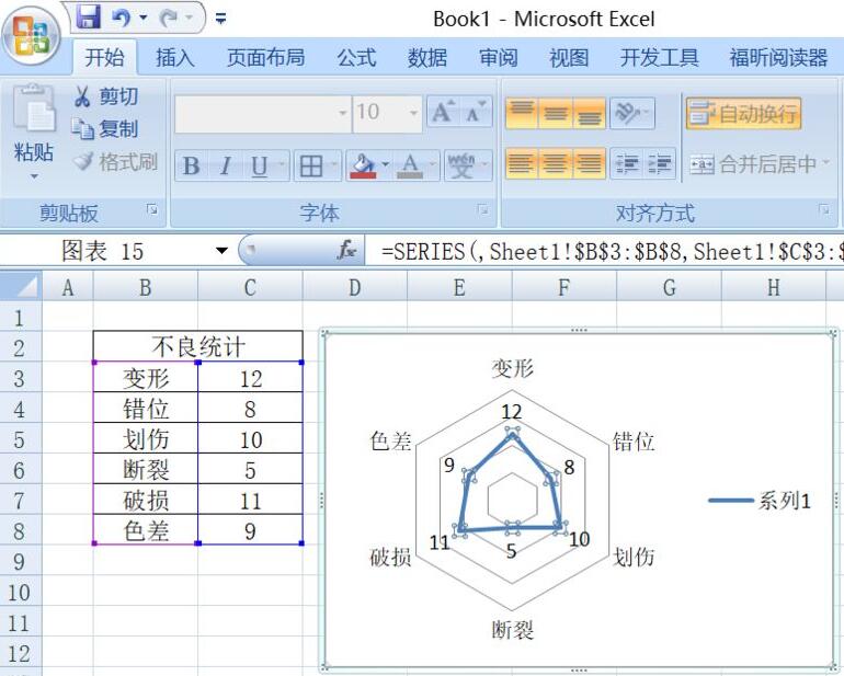
Click to select the inner value ring, as shown in the figure;
Right-click and select Add Data Label; in this way, you can see at a glance which defect has the most defects and which defect has the least.
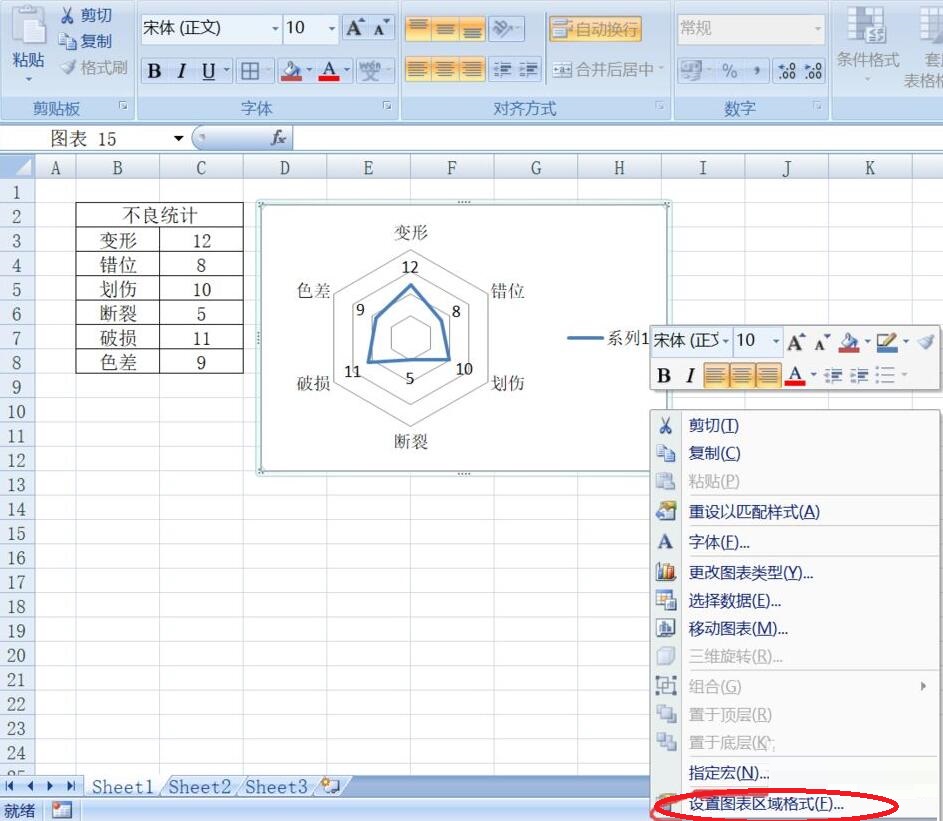
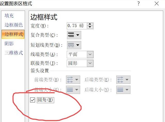
Select the chart, right-click and select Format Chart Area;
Select the border style and check Rounded Corners, then select Off;
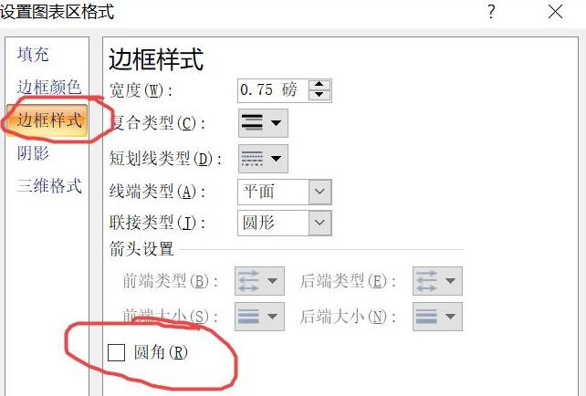
Finally, the radar chart is completed.
The above is the tutorial on inserting radar chart into office2007 Excel brought by the editor. Don’t miss it.